PSI vs. SPY: 20-Year Cumulative Return Analysis

Author

Nathan Renzoni

Published

December 31, 2020

PSI vs. SPY: 20-Year Cumulative Return Analysis (1999–2021)

This notebook compares the monthly returns of the PSI (Kirshenbaum) strategy against an SPY buy-and-hold benchmark over roughly twenty years. Using bootstrap (with and without replacement) and permutation of the return-difference series, it characterizes the distribution of 20-year cumulative returns and assesses whether PSI’s outperformance is structurally robust or merely timing-dependent.

Data note. The Kirsh monthly returns (1999-12-31 → 2021-12-31, 259 months) were pre-computed in a separate notebook and are loaded from a pickle. SPY daily closes are loaded from a materialized parquet (sourced from the daily_ohlc Postgres table); that table currently ends 2021-07-09, so the joined analysis covers 1999-12 to 2021-07 (254 months).

Setup

from trading_research.research_setup import *  # pd, np, plt, AnalysisCore, Path, ...
import seaborn as sns
import re
plt.rcParams["figure.figsize"] = [15, 5]
plt.rcParams['figure.dpi'] = 110
plt.rcParams['savefig.dpi'] = 150
sns.set_theme()

importing stock_data_dealer
importing stock_data_dealer.db
importing stock_data_dealer.models
importing stock_data_dealer.utils
importing stock_data_dealer.enums
importing stock_data_dealer.models_utils
importing stock_data_dealer.premarket
importing stock_data_dealer.controllers
importing stock_data_dealer.parsers
importing stock_data_dealer.iqfeed_io
loading .env from /home/trade/Dev/trading-research/.env

Strategy returns (Kirsh / PSI)

# data pre-processed in a different notebook (monthly PSI/Kirsh strategy returns)
kirsh_ret_df = pd.read_pickle('kirsh_ret_df_1999_to_2021.pkl')

kirsh_ret_df

	start_date	end_date	period_ret	cum_ret
0	1999-12-31	2000-01-31	-0.0146	-0.0146
1	2000-01-31	2000-02-29	0.1225	0.1062
2	2000-02-29	2000-03-31	-0.0041	0.1016
3	2000-03-31	2000-04-30	-0.0534	0.0428
4	2000-04-30	2000-05-31	-0.0507	-0.0101
...	...	...	...	...
254	2021-07-31	2021-08-31	0.0267	2.7830
255	2021-08-31	2021-09-30	-0.0482	2.6005
256	2021-09-30	2021-10-31	0.0767	2.8766
257	2021-10-31	2021-11-30	0.0091	2.9118
258	2021-11-30	2021-12-31	-0.0046	2.8938

259 rows × 4 columns

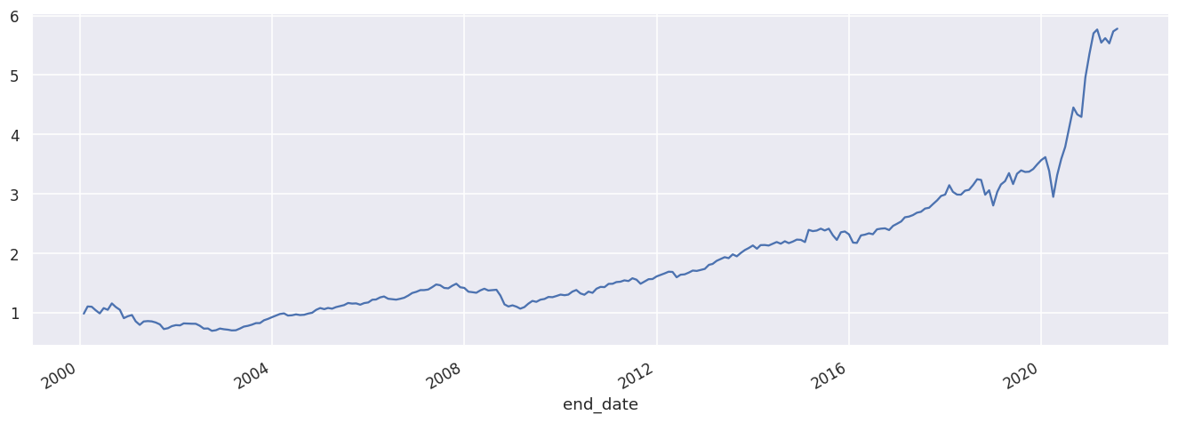
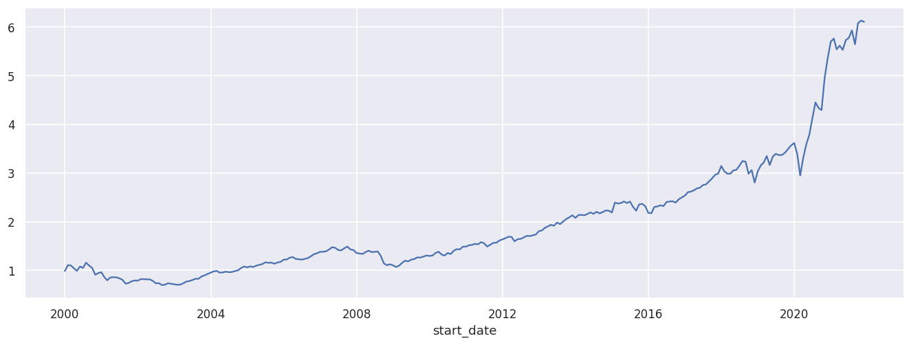
Cumulative growth of $1 in the PSI strategy, indexed by period start date.

kirsh_ret_df.set_index('start_date', drop=False).period_ret.add(1).cumprod().plot();

kirsh_start_date = kirsh_ret_df.start_date[0]
kirsh_end_date = kirsh_ret_df.end_date.iloc[-1]

SPY benchmark

# SPY daily closes materialized from the daily_ohlc Postgres table
# (self-contained so the notebook renders without a live DB at build time).
# Note: SPY data in Postgres ends 2021-07-09; analysis covers 1999-12 to 2021-07.
spy_ret = pl.read_parquet('spy_daily_close_1999_to_2021.parquet')

spy_daily_ret_df = spy_ret.to_pandas()

spy_monthly_ret = spy_daily_ret_df.set_index('date')
spy_monthly_ret.index = pd.DatetimeIndex(spy_monthly_ret.index)
spy_monthly_ret = spy_monthly_ret.pct_change().add(1).resample('ME').prod().sub(1)
spy_monthly_ret.columns = ['spy_month_ret']

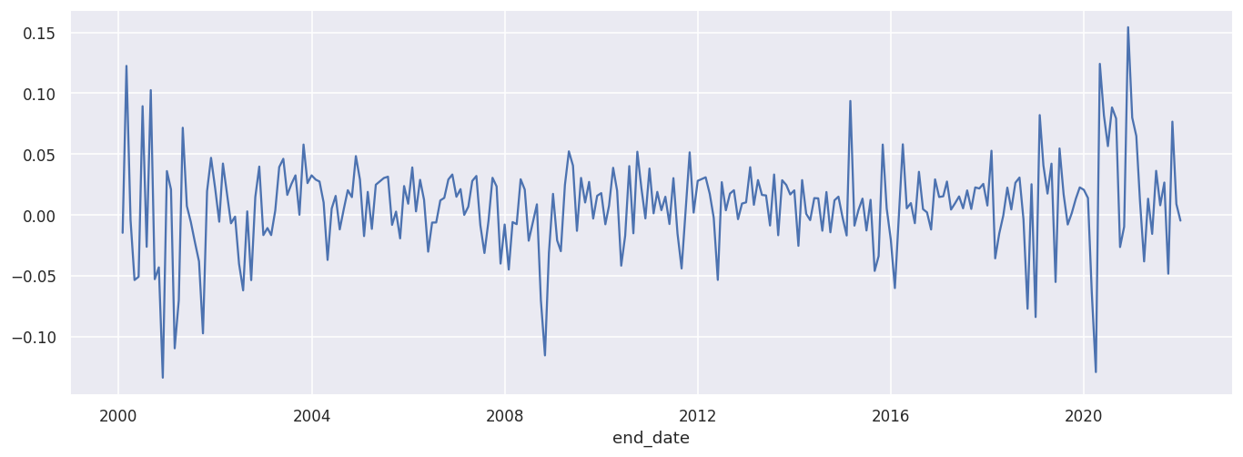
PSY monthly returns by end_date (Kirsh), for visual comparison with SPY below.

kirsh_ret_df.set_index('end_date').period_ret.plot();

spy_monthly_ret

	spy_month_ret
date
1999-12-31	0.044402
2000-01-31	-0.048268
2000-02-29	-0.015226
2000-03-31	0.094134
2000-04-30	-0.035120
...	...
2021-03-31	0.037780
2021-04-30	0.064170
2021-05-31	-0.000048
2021-06-30	0.018236
2021-07-31	0.007529

260 rows × 1 columns

Join Kirsh and SPY monthly returns on end_date.

both_ret_df = kirsh_ret_df.set_index('end_date').join(spy_monthly_ret)[['period_ret', 'spy_month_ret']].dropna()
both_ret_df.columns = ['kirsh', 'spy']

both_ret_df

	kirsh	spy
end_date
2000-01-31	-0.0146	-0.048268
2000-02-29	0.1225	-0.015226
2000-03-31	-0.0041	0.094134
2000-04-30	-0.0534	-0.035120
2000-05-31	-0.0507	-0.015723
...	...	...
2021-03-31	-0.0381	0.037780
2021-04-30	0.0134	0.064170
2021-05-31	-0.0155	-0.000048
2021-06-30	0.0363	0.018236
2021-07-31	0.0080	0.007529

254 rows × 2 columns

Per-year and full-period comparison

def plot_return_series_for_year(year):
    both_ret_df[str(year):str(year+1)].add(1).cumprod().plot()
    
def get_return_series_for_year(year):
    return both_ret_df[str(year):str(year+1)].add(1).cumprod().iloc[-1]

Year-end cumulative returns, Kirsh vs SPY, 2000→2021.

pd.DataFrame([get_return_series_for_year(i) for i in range(2000, 2021+1)])

	kirsh	spy
2001-12-31	0.792421	0.779457
2002-12-31	0.767013	0.652758
2003-12-31	1.168968	0.944929
2004-12-31	1.493830	1.369942
2005-12-31	1.267183	1.083959
2006-12-31	1.252619	1.135094
2007-12-31	1.208238	1.174283
2008-12-31	0.831973	0.642976
2009-12-31	0.920595	0.769102
2010-12-31	1.320851	1.393506
2011-12-31	1.234736	1.216439
2012-12-31	1.169433	1.169050
2013-12-31	1.322676	1.406412
2014-12-31	1.281079	1.443298
2015-12-31	1.088007	1.103850
2016-12-31	1.121992	1.087526
2017-12-31	1.288206	1.308971
2018-12-31	1.122683	1.118060
2019-12-31	1.193977	1.206101
2020-12-31	1.908913	1.488436
2021-07-31	1.619610	1.338843
2021-07-31	1.079383	1.158418

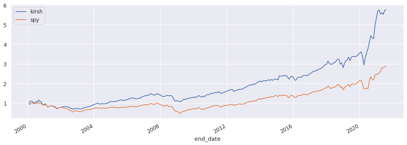
Full-period cumulative growth of $1: Kirsh vs SPY.

both_ret_df.add(1).cumprod().plot();

both_ret_df['2020':].add(1).cumprod().sub(1).iloc[-1]

kirsh    0.619610
spy      0.338843
Name: 2021-07-31 00:00:00, dtype: float64

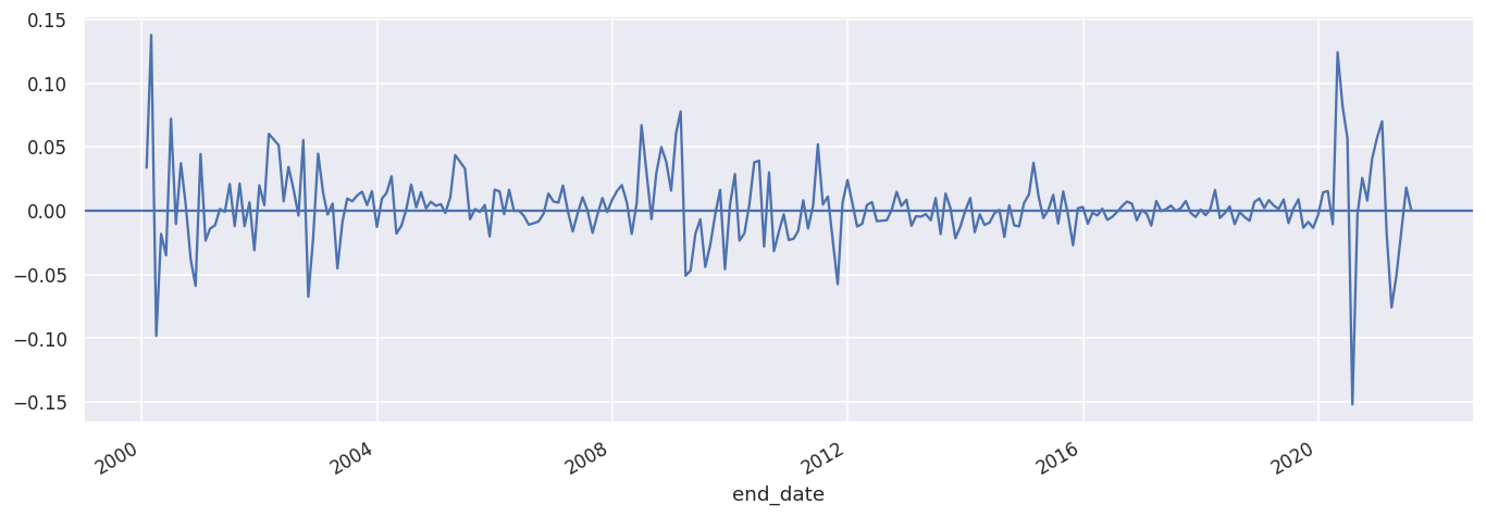
Kirsh minus SPY monthly return difference. Positive = PSI outperformed SPY that month.

ret_diff_series = both_ret_df['kirsh'] - both_ret_df['spy']
ret_diff_series.plot()
plt.axhline(0);

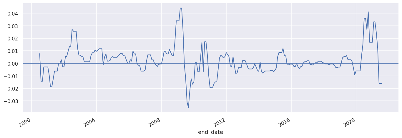
6-month rolling median of the return difference — smooths month-to-month noise.

ret_diff_series.rolling(6).median().plot()
plt.axhline(0);

Distribution of return differences

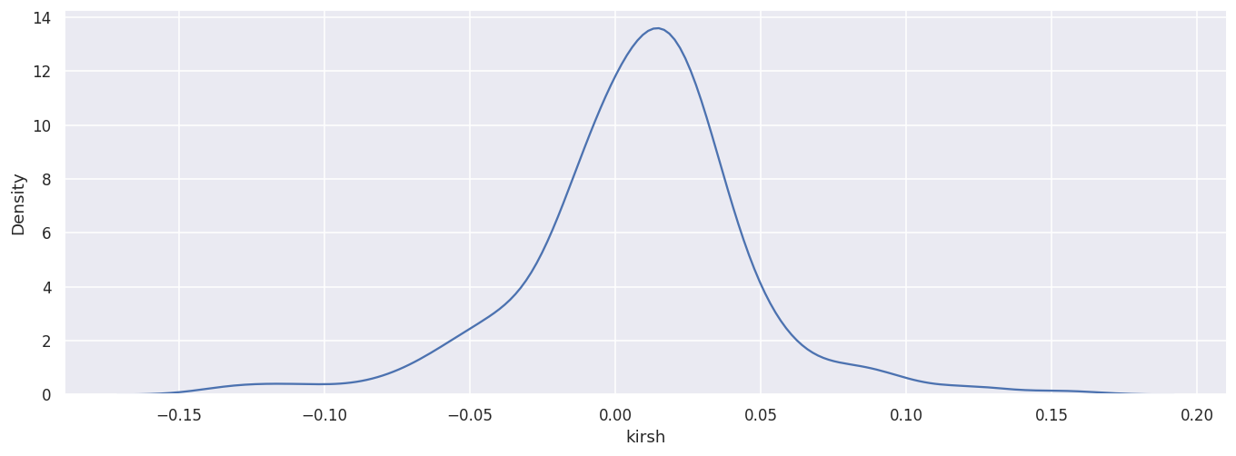
Density of Kirsh monthly returns.

sns.kdeplot(both_ret_df['kirsh']);

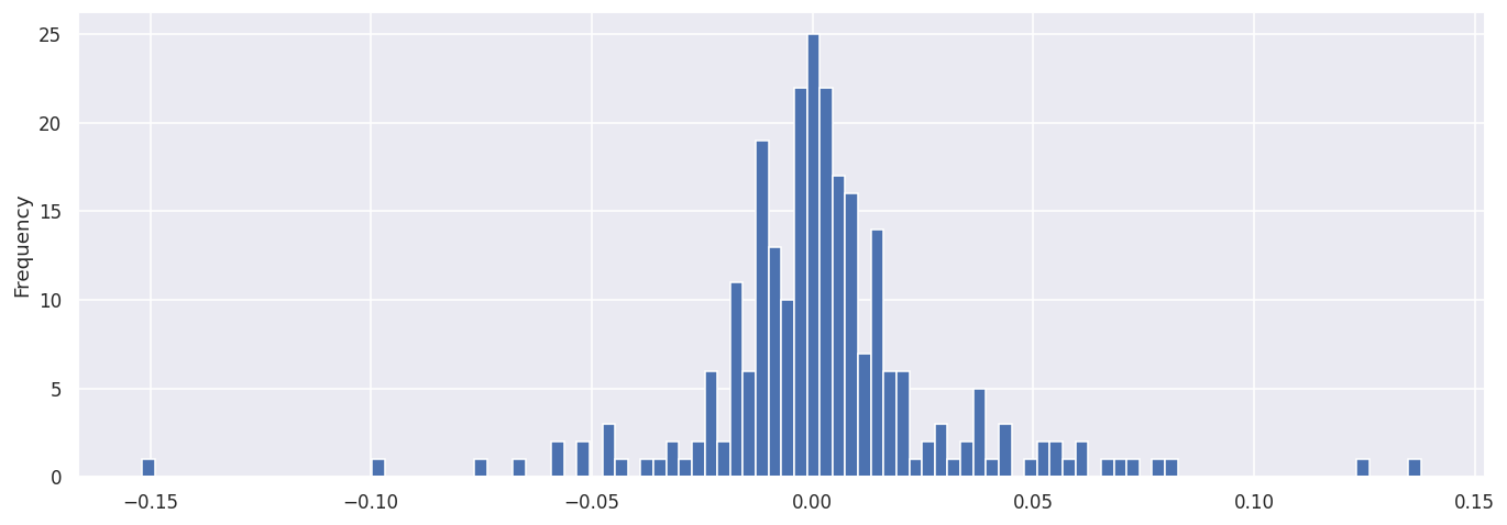
Histogram of (Kirsh − SPY) monthly return differences.

ret_diff_series.plot.hist(bins=100);

ret_diff_series.values

array([ 3.36683513e-02,  1.37726153e-01, -9.82336971e-02, -1.82798005e-02,
       -3.49770677e-02,  7.21129978e-02, -1.03973597e-02,  3.72587413e-02,
        4.53107865e-03, -3.83218451e-02, -5.89475441e-02,  4.43687424e-02,
       -2.34592663e-02, -1.41124653e-02, -1.14279952e-02,  1.25694575e-03,
       -9.25994716e-04,  2.08978563e-02, -1.21042414e-02,  2.12325093e-02,
       -1.21364871e-02,  6.57816928e-03, -3.09773157e-02,  1.99079790e-02,
        4.29877515e-03,  6.02360311e-02,  5.13557806e-02,  7.41500093e-03,
        3.43481856e-02,  1.69197251e-02, -3.80122861e-03,  5.53472434e-02,
       -6.74838978e-02, -2.18809761e-02,  4.46832305e-02,  1.38948090e-02,
       -3.02103184e-03,  5.58457008e-03, -4.52117536e-02, -8.63625286e-03,
        9.48607530e-03,  7.37275428e-03,  1.19741825e-02,  1.48884858e-02,
        4.37323662e-03,  1.52788224e-02, -1.27734147e-02,  9.33005032e-03,
        1.39293268e-02,  2.69927491e-02, -1.79786914e-02, -1.18232877e-02,
        9.02906256e-04,  2.04186327e-02,  2.66405630e-03,  1.45499415e-02,
        1.81524696e-03,  6.96890459e-03,  3.82219866e-03,  5.12078266e-03,
       -1.90385917e-03,  1.07337976e-02,  4.36351645e-02,  3.29108805e-02,
       -6.76145326e-03,  1.27449491e-03, -9.52651330e-04,  4.45084525e-03,
       -2.01523849e-02,  1.64764612e-02,  1.50858646e-02, -2.72549020e-03,
        1.64224207e-02, -1.31903258e-04,  2.09401384e-05, -4.00409380e-03,
       -1.09730645e-02, -9.82244818e-03, -8.40459277e-03, -2.31669412e-03,
        1.34146672e-02,  7.24364904e-03,  6.25975145e-03,  1.97173913e-02,
       -6.92421770e-04, -1.62957746e-02, -1.82002158e-03,  1.05494652e-02,
        1.10243967e-04, -1.74328301e-02, -3.20987872e-03,  9.93334644e-03,
       -1.16737795e-03,  8.68055967e-03,  1.56609808e-02,  2.00426148e-02,
        6.32454043e-03, -1.82623475e-02,  5.78355273e-03,  6.70368009e-02,
       -6.65375700e-03,  2.94865983e-02,  4.98866540e-02,  3.85065269e-02,
        1.57349983e-02,  6.13143617e-02,  7.77489919e-02, -5.09120655e-02,
       -4.70460765e-02, -1.78534431e-02, -6.73176267e-03, -4.41057640e-02,
       -2.66395810e-02, -3.34850673e-03,  1.63253054e-02, -4.58067980e-02,
        4.35619429e-03,  2.87424264e-02, -2.34947109e-02, -1.77288062e-02,
        4.50854701e-03,  3.78823777e-02,  3.92225128e-02, -2.81007169e-02,
        2.99805024e-02, -3.17527300e-02, -1.63020503e-02, -2.82109883e-03,
       -2.30486022e-02, -2.19001988e-02, -1.57373329e-02,  8.20578295e-03,
       -1.39614601e-02,  3.81454226e-03,  5.20197924e-02,  4.80454649e-03,
        1.10756437e-02, -5.76471498e-02,  6.06374502e-03,  2.40196736e-02,
       -1.24054219e-02, -1.02601956e-02,  4.47566224e-03,  6.75576607e-03,
       -8.25519130e-03, -7.89236619e-03, -7.45264687e-03,  4.93510910e-04,
        1.47982357e-02,  3.70491687e-03,  8.60618339e-03, -1.18902254e-02,
       -4.35885104e-03, -4.67510718e-03, -2.71235718e-03, -7.47840681e-03,
        9.90775490e-03, -1.83768483e-02,  1.33922945e-02,  1.95777574e-03,
       -2.16067675e-02, -1.27376358e-02, -8.67403315e-05,  9.94825383e-03,
       -1.68157706e-02, -2.86494176e-03, -1.11514999e-02, -9.30641495e-03,
       -2.07745485e-03,  5.37563867e-04, -2.05634626e-02,  4.18473419e-03,
       -1.14509085e-02, -1.23719825e-02,  6.01158301e-03,  1.28292692e-02,
        3.74954375e-02,  1.13797494e-02, -5.83384198e-03,  6.43816560e-04,
        1.23544662e-02, -1.00892640e-02,  1.50501188e-02, -3.14402287e-03,
       -2.71597506e-02,  1.84492377e-03,  2.89645886e-03, -1.02172953e-02,
       -1.66993942e-03, -3.68962596e-03,  1.55488517e-03, -7.20764016e-03,
       -4.96057949e-03, -9.96001910e-04,  3.60250553e-03,  7.16825835e-03,
        5.43703190e-03, -7.53839097e-03,  5.06506943e-04, -2.49468975e-03,
       -1.17915220e-02,  7.58707236e-03, -3.26189870e-04,  1.18709677e-03,
        4.00894632e-03, -3.54177006e-04,  2.08230336e-03,  7.58827831e-03,
       -1.76406480e-03, -4.96581762e-03,  8.19131354e-04, -3.55913962e-03,
        7.60411493e-04,  1.61902632e-02, -5.76815504e-03, -1.80909984e-03,
        3.34510962e-03, -1.05465939e-02, -1.11980948e-03, -4.91228342e-03,
       -7.89570721e-03,  6.75068913e-03,  9.54300744e-03,  2.03437900e-03,
        8.28418849e-03,  3.96428879e-03,  1.34755027e-03,  8.77117203e-03,
       -9.70948887e-03,  1.78054608e-03,  8.94343543e-03, -1.33717559e-02,
       -8.80466017e-03, -1.34982000e-02, -3.32087111e-03,  1.44039023e-02,
        1.53657601e-02, -1.06580031e-02,  1.24200000e-01,  8.18000000e-02,
        5.66000000e-02, -1.51875651e-01, -2.87063835e-03,  2.56424953e-02,
        7.94069260e-03,  4.05926441e-02,  5.71221162e-02,  7.00614291e-02,
       -1.67055503e-02, -7.58799979e-02, -5.07704456e-02, -1.54523878e-02,
        1.80636416e-02,  4.71358429e-04])

Random SPY sample (12 × 20 months) cumulative product — a random-walk sanity check.

pd.Series(np.random.choice(both_ret_df['spy'], 12*20)).add(1).cumprod().plot();

Bootstrap methodology

Permutation / sampling helpers used to build the bootstrap ensembles below.

def permute_columns(x):
    ix_i = np.random.sample(x.shape).argsort(axis=0)
    ix_j = np.arange(x.shape[1])
    return x[ix_i, ix_j]

def permute_rows(x):
    ix_i = np.arange(x.shape[0]).reshape(-1,1)
    ix_j = np.random.sample(x.shape).argsort(axis=1)
    return x[ix_i, ix_j]

def choose_rand_rows(x):
    ix_i = np.arange(x.shape[0]).reshape(-1,1)
    ix_j = np.random.randint(0, x.shape[1], size=x.shape)
    return x[ix_i, ix_j]

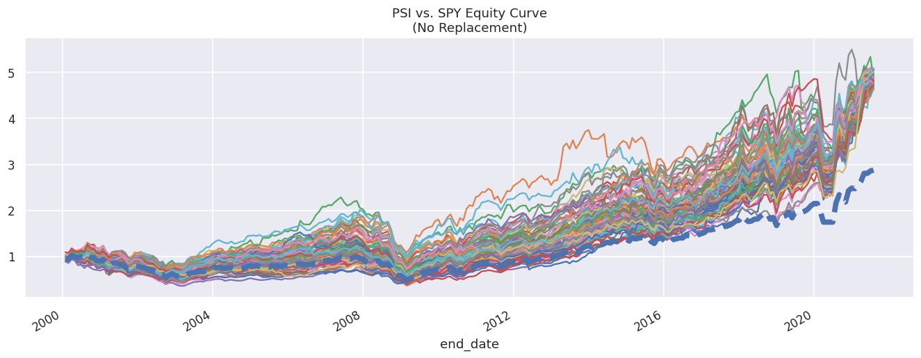
Build the ensembles: - No replacement: permute the order of the (Kirsh − SPY) difference series, re-add it to SPY, and compound — tests whether PSI’s timing matters. - With replacement: resample Kirsh and SPY monthly returns independently (1000 draws each) and compound — characterizes the distribution of 20-year outcomes under each strategy.

permuted_ret_diff_series_arr = permute_rows(
    np.tile(ret_diff_series, (100,1))
)
kirsh_rand_choice_series_arr = choose_rand_rows(
    np.tile(both_ret_df['kirsh'], (1_000,1))
)

spy_rand_choice_series_arr = choose_rand_rows(
    np.tile(both_ret_df['spy'], (1_000, 1))
)

kirsh_ret_bootstrap_no_replacement_df = pd.DataFrame(
    (permuted_ret_diff_series_arr + both_ret_df['spy'].values + 1).cumprod(1).T,
    index=both_ret_df.index)

kirsh_ret_bootstrap_replacement_df = pd.DataFrame(
    (kirsh_rand_choice_series_arr + 1).cumprod(1).T,
    index=both_ret_df.index)

spy_ret_bootstrap_replacement_df = pd.DataFrame(
    (spy_rand_choice_series_arr + 1).cumprod(1).T,
    index=both_ret_df.index
)

spy_final_ret = both_ret_df['spy'].add(1).cumprod().iloc[-1]

Results

Bootstrap (no-replacement) equity curves vs the actual SPY buy-and-hold (dashed). Tests timing sensitivity.

fig, ax = plt.subplots(1)

kirsh_ret_bootstrap_no_replacement_df.plot(ax=ax);
both_ret_df['spy'].add(1).cumprod().plot(style='--', linewidth=5, ax=ax, label=None)
ax.legend().remove()
ax.title.set_text('PSI vs. SPY Equity Curve\n(No Replacement)');

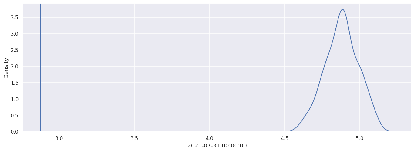
Density of no-replacement final returns; red line = actual SPY 20-year final return.

sns.kdeplot(kirsh_ret_bootstrap_no_replacement_df.iloc[-1])
plt.axvline(spy_final_ret);

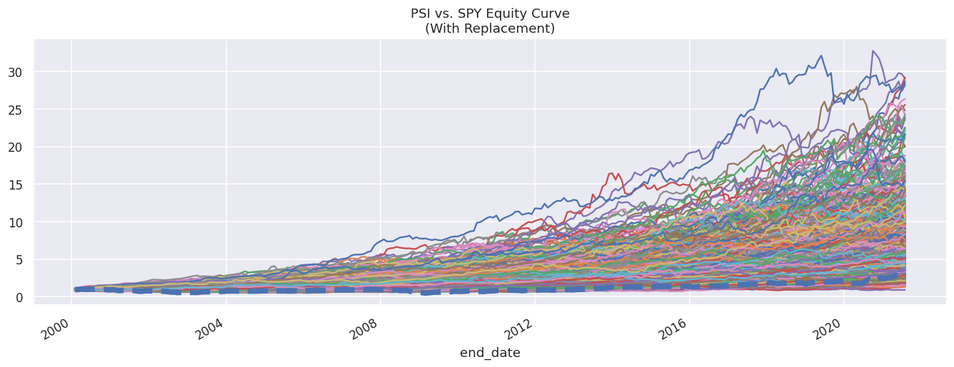
Bootstrap (with-replacement) equity curves vs actual SPY (dashed).

kirsh_ret_bootstrap_replacement_df.plot(legend=False);
both_ret_df['spy'].add(1).cumprod().plot(style='--', linewidth=5)
plt.title('PSI vs. SPY Equity Curve\n(With Replacement)');

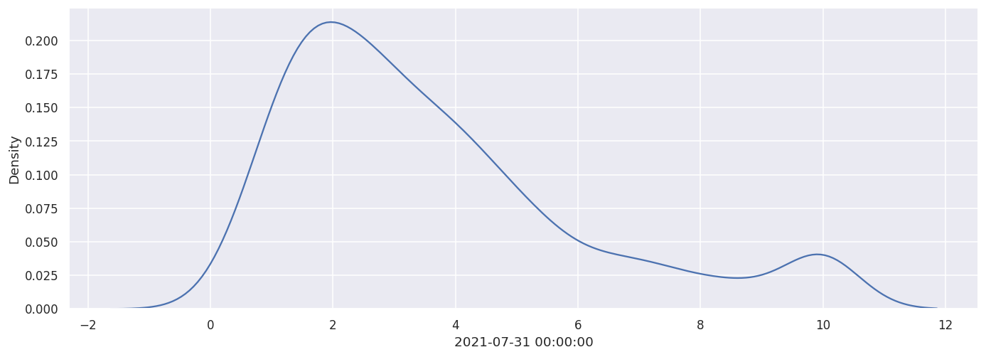
Density of SPY with-replacement final returns (clipped 0–10).

sns.kdeplot(
    spy_ret_bootstrap_replacement_df.iloc[-1]\
        .clip(0, 10),
#     bw_adjust=1.9,
    label='SPY with replacement'
);

spy_ret_bootstrap_replacement_df.iloc[-1].median(), kirsh_ret_bootstrap_replacement_df.iloc[-1].median()

(np.float64(2.9539108947013006), np.float64(5.721996800838706))

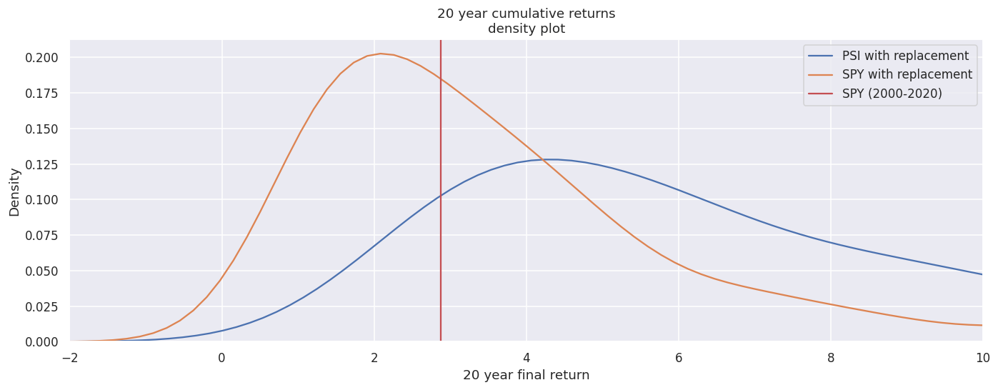
Dual density: Kirsh vs SPY with-replacement 20-year final returns. Red line = actual SPY.

sns.kdeplot(
    kirsh_ret_bootstrap_replacement_df.iloc[-1]\
        .rename(),
    label='PSI with replacement'
)
sns.kdeplot(
    spy_ret_bootstrap_replacement_df.iloc[-1]\
        .rename(),
#     bw_adjust=1.9,
    label='SPY with replacement'
)

plt.xlim(-2,10)

plt.axvline(both_ret_df['spy'].add(1).cumprod().iloc[-1], color='r', label='SPY (2000-2020)')
plt.title('20 year cumulative returns\ndensity plot')
plt.xlabel('20 year final return')
plt.legend();

A single permutation of the difference series re-added to SPY — what a randomized PSI timing sequence looks like.

(pd.Series(
    np.random.permutation(ret_diff_series.values),
    index=ret_diff_series.index) + both_ret_df['spy']).add(1).cumprod().plot()

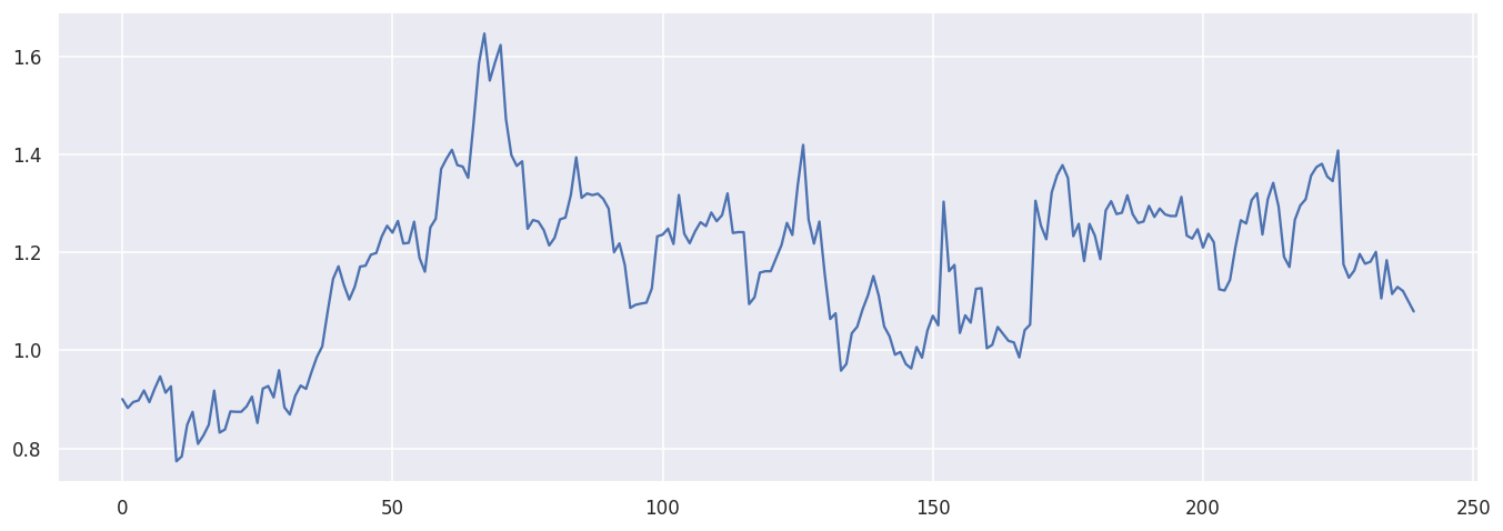
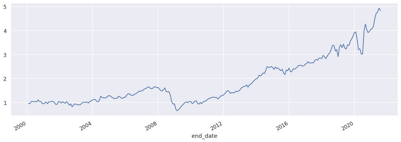
The actual (Kirsh − SPY) + SPY sequence compounded — PSI’s real timing.

(ret_diff_series + both_ret_df['spy']).add(1).cumprod().plot()